library(httr)
library(jsonlite)
library(dplyr)
library(fpp2)
library(quantmod)
library(tidyquant)

api_key = "YOUR_API_KEY"Excess Return Model In R
Equity Research
CAPM
R
Excess Return
Making financial institution valuations easy and fast with R.
Problem with Valuations of Financial Institutions
You’re diligently constructing a “diversified” stock portfolio, conducting thorough analyses, constructing DCF models, statistical models, and meticulously organizing data in spreadsheets. All seems well until the moment you consider adding some financials to your portfolio. Unintentionally, you might subject JP Morgan or Goldman through your well-established and trusted DCF model, only to encounter chaos. Is the data flawed? Is there an issue with my model? Fortunately, the likely answer to both queries is no. Instead, it boils down to a few technical and practical reasons why valuing financial institutions with firm value becomes challenging. I won’t delve into every detail, but essentially, we encounter four distinct reasons why a DCF model and similar firm value models struggle in this scenario.
Firstly, regulatory constraints demand that banks meet minimum capital requirements, often linked to the book value of equity and operations. These constraints and the potential tightening of regulations can diminish reinvestment ability and subsequently stifle growth. Hence, investors and analysts must comprehend the regulatory structures governing their positions in financial institutions.
Secondly, the unique business model and accounting principles of financial institutions make traditional valuation approaches challenging. Mark-to-market, a standard practice for recording assets at their current fair value rather than their acquisition cost, is distinct for FIs compared to most non-FIs that record assets at cost. Since FIs hold a significantly higher proportion of market securities, these assets are often not held to maturity due to liquidity rules and the nature of their business. Consequently, the implication for valuations is that the book value of equity for an FI reflects its current equity value, unlike non-FIs where the book value of equity represents total equity investment and ROE measures return on that investment.
Thirdly, while traditional firms raise capital through debt and equity sales so, determining the total cost of capital (WACC) is integral step in evaluating a firm’s growth and operational maintenance costs. However, for FIs, debt disproportionately outweighs equity furthermore, it challenging to discern what types of debt to include in an analysis, deposits, savings accounts, short term/long term bond sales. This disproportionately skewed cost of capital often falls around 5-4% due to banks utilizing debt more as “raw material” than capital, using it to make and lend more money at higher rates than it pays to borrow. For analysts, this high debt load and distorted cost of capital can disrupt traditional models.
Lastly, DCF and firm valuation models struggle due to the nature of cash flows in FIs. Firstly, unlike manufacturing companies, capital expenditures and associated depreciation are often negligible for FIs. Secondly, the working capital account, defined by current assets less current liabilities, tends to be substantial and significantly changes as the banks’ positions fluctuate, making forecasting nearly impossible.
For a more detailed explanation into why the DCF fails at valuing financial institutions check out this chapter from Aswath Damodaran’s Darkside of Valuations.
Excess Return Model
Now it is clear that we need an alternative to firm valuation models. This is where our discussion on the Excess Return Model begins. First, we will briefly explain the mechanics and then delve into how to implement it in R. This includes everything from gathering the data from the Financial Modeling Prep API to manipulating, cleaning, and calculating the data to ultimately arrive at a fair value per share.
\[ExcessEquityReturn = (ReturnOnEquity – CostOfEquity)*(EquityCapitalInvested)\] Lets break down this formula.
Return on Equity - A forecast for the future economic benefit (net income) divided by the current book value of shareholders equity.
Cost of Equity - Similar to most models is measured by the Capital Asset Pricing Model
\(Cost of Equity = RiskFreeRate + Beta * (Market Risk Premium)\)
Equity Capital Invested - The current book value of shareholder equity invested.
Getting Started In R
The previous formula was quite straightforward in explaining how to calculate the excess return. However, transitioning from the formula to a fair value estimate requires a few more steps. So, let’s delve into how we can convert the excess return formula into a forecast, determine the present value of all future returns, and arrive at a fair value estimate. And what better way to illustrate this process than by walking through the code!
For this project, we’ll depend on several R packages that, in my experience, work well together and allow us to accomplish some impressive tasks. However, the most crucial resource we’ll rely on is the API from Financial Modeling Prep. If you’ve never used it before, I highly recommend it. They offer a free tier with five years of data, but for this project, I’m utilizing a paid for starter plan, providing access to thirty-plus years of data, so your experience may vary if you use the free tier. Nonetheless, they provide a much more reliable and robust method to extract financial data compared to other R packages… in my experience.
Function Junction!
I love functions, so get ready! There are several needed for this project, but the good news is they are all pretty similar, just calling the API and returning a dataframe. The exception is the “getBeta()” function, which calculates the regression beta… sorry, Professor Damodaran.
#------------------FUNCTIONS---------------------

#BALANCE SHEET
getBS <- function(stock_symbol, limit, api_key) {
  base_url <- paste0("https://financialmodelingprep.com/api/v3/balance-sheet-statement/", stock_symbol, "?period=quarterly&limit=", limit,"&apikey=", api_key)

  response <- GET(base_url)

  data <- content(response, "text", encoding = "UTF-8")
  data <- jsonlite::fromJSON(data)
  data <- as.data.frame(data)
  data
}

#INCOME STATEMENT
getIS <- function(stock_symbol, limit, api_key) {
  base_url <- paste0("https://financialmodelingprep.com/api/v3/income-statement/", stock_symbol, "?period=quarterly&limit=", limit,"&apikey=", api_key)

  response <- GET(base_url)

  data <- content(response, "text", encoding = "UTF-8")
  data <- jsonlite::fromJSON(data)
  data <- as.data.frame(data)
  data
}

#METRICS
getMetrics <- function(stock_symbol, limit, api_key) {
  base_url <- paste0("https://financialmodelingprep.com/api/v3/key-metrics/", stock_symbol, "?period=quarterly&limit=", limit,"&apikey=", api_key)

  response <- GET(base_url)

  data <- content(response, "text", encoding = "UTF-8")
  data <- jsonlite::fromJSON(data)
  data <- as.data.frame(data)
  data
}

#RATES
getRates <- function(start, end, api_key) {
  base_url <- paste0("https://financialmodelingprep.com/api/v4/treasury?from=", start, "&to=", end, "&apikey=", api_key)

  response <- GET(base_url)

  data <- content(response, "text", encoding = "UTF-8")
  data <- jsonlite::fromJSON(data)
  data <- as.data.frame(data)
  data
}

#BETA
getBeta <- function(stock_symbol, api_key) {

  # 1) Get price data on company
  base_url <- paste0("https://financialmodelingprep.com/api/v3/historical-price-full/", stock_symbol, "?apikey=", api_key)
  response <- GET(base_url)
  data <- content(response, "text", encoding = "UTF-8")
  data <- jsonlite::fromJSON(data)
  data <- as.data.frame(data)
  data <- data %>% arrange(desc(row_number())) #order from oldest to latest price
  stock_returns <- diff(log(data$historical.adjClose)) #calculate the log returns
  stock_returns <- as.data.frame(stock_returns)


  # 2) Get S&P Returns
  base_url <- paste0("https://financialmodelingprep.com/api/v3/historical-price-full/SPY?apikey=", api_key)
  response <- GET(base_url)
  data <- content(response, "text", encoding = "UTF-8")
  data <- jsonlite::fromJSON(data)
  data <- as.data.frame(data)
  data <- data %>% arrange(desc(row_number())) #order from oldest to latest price
  spy_returns <- diff(log(data$historical.adjClose)) #calculate the log returns
  spy_returns <- as.data.frame(spy_returns)

  df <- cbind(stock_returns, spy_returns)
  colnames(df) <- c("Stock_Returns", "SPY_Returns")
  model <- lm(Stock_Returns ~ SPY_Returns, data = df)
  beta <- coef(model)[2]  # Extract the beta coefficient
  beta <- as.double(beta)
}

#MARKET PREMIUM
getPremium <- function(stock_symbol, limit, api_key) {
  base_url <- paste0("https://financialmodelingprep.com/api/v3/key-metrics/", stock_symbol, "?period=annual&limit=", limit,"&apikey=", api_key)

  response <- GET(base_url)

  data <- content(response, "text", encoding = "UTF-8")
  data <- jsonlite::fromJSON(data)
  data <- as.data.frame(data)
  data
}
Okay great now we have a data pipeline, and even better we can easily reuse the functions for later projects!
Set Function Parameters
#-------------------PARAMETERS--------------------
#Set the target company Ticker
target="JPM"

# Set forecast length
h=10

# Set historical data length
hist_h=10
Get Book Value of Shareholder Equity
Firstly, obtain the book value of shareholder equity from the balance sheet and rearrange the data using the “arrange()” method in R, reordering the dataframe from the oldest to the latest book value. Then visualize the change over the quarters. However, what we’re really after is the “bv_of_equity_current”—also known as the book value of shareholder equity. It is the first input needed for the excess return model and is the starting point to later calculate the excess returns and future book value of equity.
#-----------------EQUITY VALUE----------------
# Get the Balance Sheet
bs <- getBS(target, hist_h, api_key)

# Assign SH Equity
equity <- bs$totalStockholdersEquity
equity <- as.data.frame(equity)
equity <- equity %>% arrange(desc(row_number()))

# Equity value over time
plot(equity$equity, type = "l", main = "Equity Value Over Time", xlab = "Quarters", ylab = "Equity Value",
     col = "#5c9a8b", lwd = 2)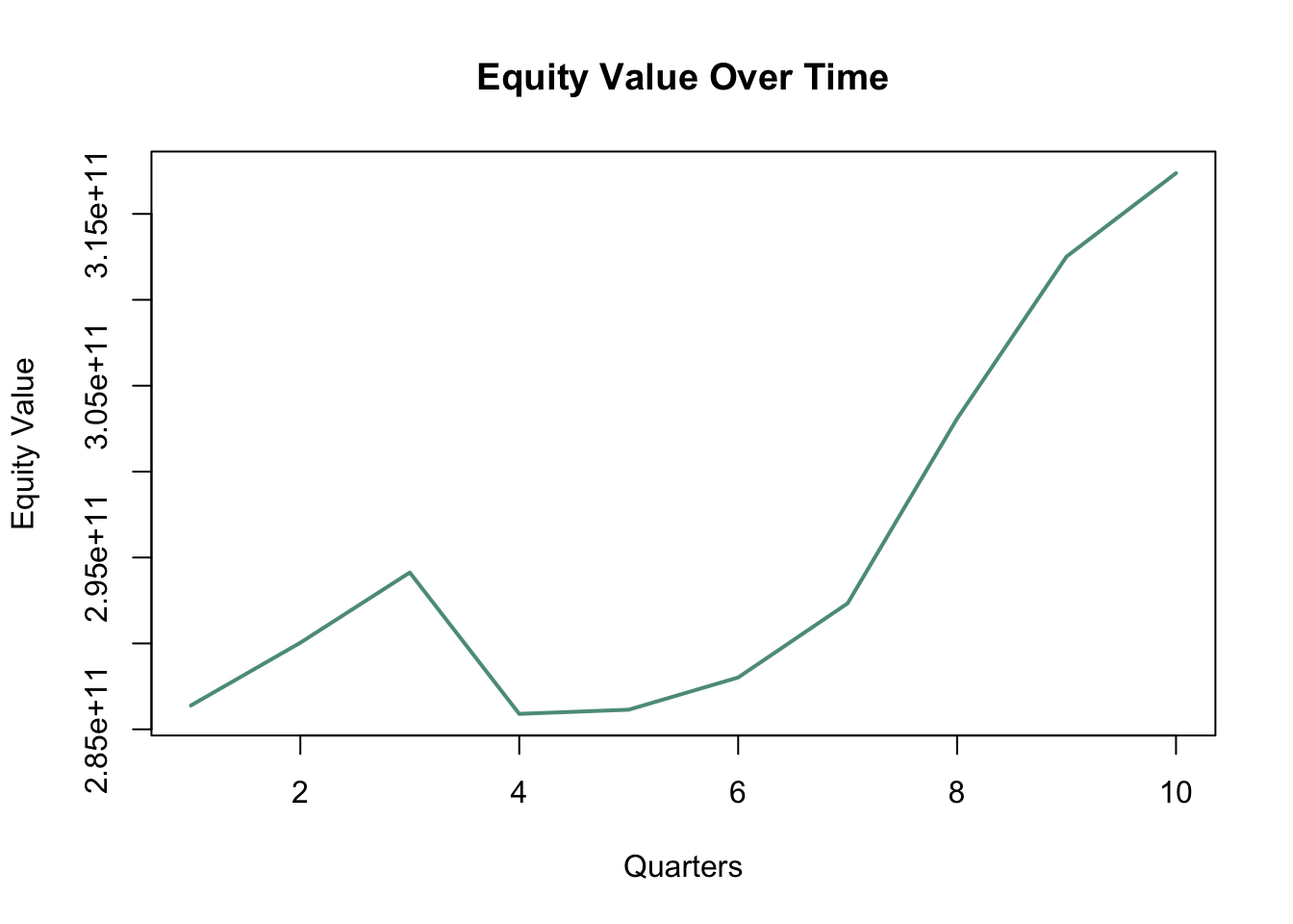
# Current book value of equity, set to h to retrieve latest bv
bv_of_equity_current <- equity$equity[h]
Get Payout Ratio
The payout ratio is percentage of income the company pays out in dividends annually, we will use this later for later calculations. But for not just know what it is. And the related Retention Ratio will be used to estimate future growth. For this demonstration I will be using the historical payout ratio as an assumption for future payout, which may not always be appropriate especially if the data being used is abnormally high or low. Adjust h, he length of data collected or set payout ratio manually. Using a filter I am able to filter out any highly unusual payout ratios which are possible when banks don’t want to cut dividends after a bad year so this helps remove the outliers. Adjust the high/low thresholds according to the box-plot output to remove outliers.
\(PayoutRatio = DividendPerShare / Earnings Per Share\)
\(Retention Ratio = 1 - PayoutRatio\)
#---------------PAYOUT RATIO----------------

# Get Metrics
key_metrics <- getMetrics(stock_symbol=target, limit=hist_h, api_key=api_key)

# Now Assign payout ratio data
payout <- key_metrics$payoutRatio

# Remove outliers from data
low_threshold <- quantile(payout, probs = 0.05, na.rm = TRUE)
high_threshold <- quantile(payout, probs = 0.95, na.rm = TRUE)
payout_filtered <- payout[payout >= low_threshold & payout <= high_threshold]

# Mean payout
payout_avg <- mean(payout_filtered)
print(payout_filtered)
[1] 0.2574709 0.2673110 0.3066860 0.3504159 0.4080537 0.3410900 0.2812361
[8] 0.2714857# Visualize & Review
boxplot(payout_filtered, main = "Payout Ratio Boxplot", xlab = "Payout Ratio",
horizontal = TRUE, col = c("#5c9a8b", "#82a8ad")) # Custom colors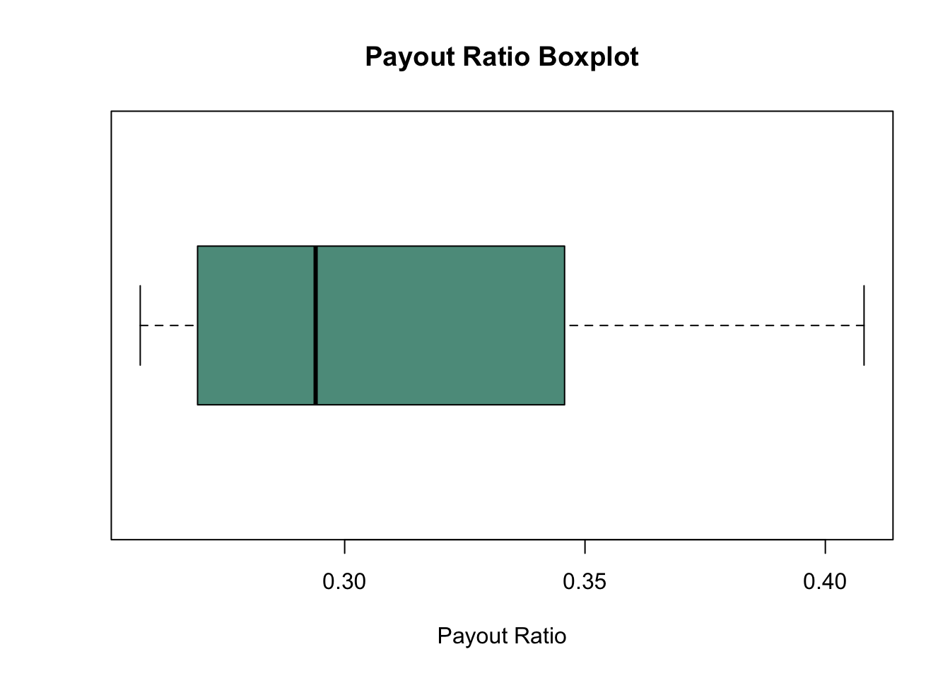
Get Cost of Capital
Much of the groundwork has already been completed using the function. Similarly, if you favor employing the bottom-up approach for calculating beta, you can substitute it at this point. For my specific requirements, I chose the automated regression approach over the bottom-up method.
#-------------------CAPM-------------------
#          COE = rf + beta*(rm-rf)

# Get Treasury Rates
rates <- getRates(start="2023-12-29", end="2023-12-29", api_key=api_key)
# Assign Risk Free Rate
rf <- rates$month3[1] /100

# Get Beta
beta <- getBeta(stock_symbol=target, api_key=api_key)

# Set market return typically between 8-12%, rm-rf = market risk premium
rm <- 0.105

# Bring it all together to calculate cost of equity
coe <- rf+beta*(rm-rf)
print(coe)
[1] 0.1106631Get Return On Equity
Similar to how we derived the payout ratio, we’re now addressing outliers, but this time through Winsorization of the data. Winsorizing serves to limit extreme values by substituting values below the lower threshold with the value at the threshold’s lower end, and likewise, values exceeding the upper threshold are replaced with the upper threshold value. This technique maintains the same number of data points while substituting extreme values. This method might prove advantageous, particularly if you later plan to forecast ROE values. Currently, we’re aggregating our quarterly values to compound an annual Return on Equity (ROE) for future use. However, it’s crucial to exercise caution while interpreting the ROE value, as past data might not accurately reflect future performance. It’s recommended to review and adjust the input for ROE accordingly to optimize results.
#-------------------ROE--------------------

# Get Income Statement
is <- getIS(target, hist_h, api_key)

# Calculate ROE
roe <- is$netIncome/bs$totalStockholdersEquity

# Winsorize extreme outliers from data
low_threshold <- quantile(roe, probs = 0.05, na.rm = TRUE)
high_threshold <- quantile(roe, probs = 0.95, na.rm = TRUE)
roe_winsorized <- pmin(pmax(roe, low_threshold), high_threshold)

roe_quarterly_avg <- mean(roe_winsorized)

# Annualized Average ROE
roe_annual_avg <- (1 + mean(roe_winsorized))^4 - 1
Forecast Excess Return
Okay now lets use that formula from the beginning to calculate the excess returns.
\[ExcessEquityReturn = (ReturnOnEquity – CostOfEquity)*(EquityCapitalInvested)\]
# Calculates Excess Return for each period of the forecast
excess_return <- c()
for (pred in seq_len(length(bv_forecast))) {
  er <- (roe_annual_avg - coe) * bv_forecast[[pred]]
  excess_return <- c(excess_return, er)
}
Terminal Growth
Here, we’re computing the growth rate for terminal value projection. Estimating growth involves considering both the Return on Equity (ROE) and the Retention Ratio, also known as the reinvestment ratio. Given that ROE gauges the return on an investment and the retention ratio signifies the portion of that return retained for reinvestment, the anticipated future growth would result from multiplying the percentage reinvested (retention ratio) by the stable return on equity.
#---------------TERMINAL GROWTH---------------

# Safety thresholds...somewhat arbitrary used as a sanity guard rail.
# If you end up hitting these thresholds you should use a different time period, or examine data for errors.
# (Expected Growth Rate = Retention ratio * Return on Equity
growth <- roe_annual_avg * (1-payout_avg)

max_growth <- 0.15
min_growth <- .025
growth <- pmin(growth, max_growth)
growth <- pmax(growth, min_growth)
Fair Value Estimation
# Calculate Terminal Value
terminal_value <- excess_return[[h]] * (1 + growth) / coe - growth
# Calculates the net present value of returns
future_returns <- c(excess_return,terminal_value)
excess_returns_npv <- NPV(cashflow=future_returns, rate=coe,)

# Calculates the total value of equity BV + Excess Returns
value_of_equity <- bv_of_equity_current + excess_returns_npv

# Get shares outstanding
shares_out <- is$weightedAverageShsOut[[1]]

# Calculates fair value per share
fair_value <- value_of_equity / shares_out
[1] "Book Value of Equity Invested Currently: 3.17371e+11"[1] "PV of Equity Excess Return: 238707231228.642"[1] "PV of Terminal Terminal Value of Excess Returns: 356270015697.623"[1] "Value of Equity: 556078231228.642"[1] "Number of Shares Outstanding: 2929561200"[1] "Value Per Share 189.816219312518"The fair value estimation of JP Morgan is .
Below are additional model results compared to the actual stock price. Each result was generated without adjusting any parameters, such as the length of historical data, market premium, risk-free rate, or maximum growth.
| Name | Ticker | Price (12/29/23) | Fair Value Projection | Price Upside/Downside |
|---|---|---|---|---|
| JP Morgan | JPM | 170.10 | 189.81 | 19.71 |
| Citi | C | 51.41 | 48.20 | -3.21 |
| Wells Fargo | WFC | 49.22 | 40.96 | -8.26 |
| Bank of America | BAC | 33.67 | 33.67 | 0.00 |
| Goldman Sachs | GS | 385.77 | 384.25 | -1.52 |
| Morgan Stanley | MS | 93.25 | 60.89 | -32.36 |
| Toronto Dominion | TD | 64.62 | 99.59 | 34.97 |
| Union Bank of Switzerland | UBS | 30.90 | 84.77 | 53.87 |
| Royal Bank of Canada | RY | 101.90 | 173.13 | 71.23 |
| US Bancorp | USB | 43.28 | 42.36 | -0.92 |
| Regions Bank | RF | 19.38 | 22.19 | 2.81 |
| Fifth Third Bancorp | FITB | 34.49 | 27.74 | -6.75 |
Fair value results compiled on 12/30/2023, stock prices pulled on 12/30/2023 based on adjusted closing prices of 12/29/2023.
Final Thoughts
The excess return model is one of those models that, by its very nature, you don’t need very often, but when you do, you really do. As the data above illustrates, either we are extremely lucky that the model produced valuations very close to the actual stock prices, or the model is exceptionally adept at capturing the true value of financial institutions. It could also be a combination of scenarios where the Excess Return model is essentially the primary method for valuing FIs, with almost every analyst using the same model and 90% of the same data, leading the valuation to become a self-fulfilling prophecy. Another intriguing observation is that, even without running any analysis, it appears that the big five banks tend to deviate less from their fair value projections. Remarkably, Bank of America’s valuation is exactly equal to the current price (I wish it was a mistake). This could be attributed to lower risk associated with these banks and/or better understanding of their risk profiles.
For future development, I would like to incorporate a more precise assessment for estimating ROE. I aim to find a way to distinguish between a bank’s stable growth and abnormal growth periods so that we can apply only the stable growth for forecasting excess returns. Additionally, I plan to implement a semi-automated bottom-up approach for beta calculation, as it has been proven to be significantly more accurate than normal regression betas.
I hope you enjoyed reading this as much as I enjoyed creating it. Most models are far more finicky than this to yield good results, so I am quite pleased with how it turned out. Feel free to message me on LinkedIn or X (Twitter) if you have any questions or if you implement any of the future development ideas—I’d love to see your work. Happy analyzing!