library(ggplot2)
ggplot(iris, aes(Petal.Length, Petal.Width, color = Species)) + geom_point()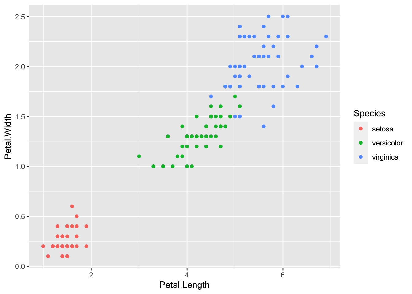
Today we will look at how to cluster data in R. For this example we will start with the well known Iris data set. But first a note on clustering.
library(ggplot2)
ggplot(iris, aes(Petal.Length, Petal.Width, color = Species)) + geom_point()
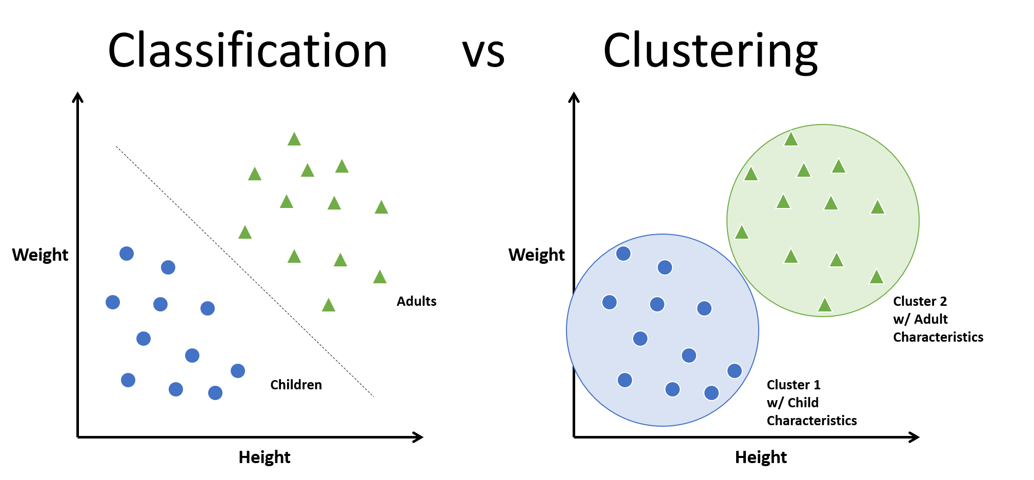
Clustering is simply grouping data points that are in proximity to other data points, i.e. grouping data that is similar or exabits similar characteristics. The most popular form of clustering for data scientists is k-means which is slightly different from the more well-known k-nn (k nearest neighbor) and the difference between the two can be subtle, but their uses are very different. K-means is a unsupervised learning and k-nn is supervised learning what that means in practice is we use k-means when the classes of the data are unknown, and we are trying to group (cluster) the data based on the distance between each observation. For k-nn we have a labeled set of data, and when we are trying to determine what class, a new unlabeled observation belongs to the algorithm simply checks which group (cluster) the observation is closest to.
The term ‘K’ refers to the number of clusters you wish to create, and R provides ways to determine the optimal number for k.
In summary k-means clusters all the observations and, k-nn classifies an observation based on its proximity to a cluster. For this Post we will focus on k-means and clustering.
K-nn = Classification
K-means = Clustering
K-means starts by determining the number of clusters K there are. Sometimes this is known before hand and sometimes you will have to use R to solve for this like the code shown below.
We are using the Iris dataset and we already know the correct number of clusters is 3 based on the three species ( setosa, virginica, versiclor), but, for illustrative purposes lets use the NbClust package in R. Which is used for determining the optimal number of clusters in a dataset by evaluating multiple indices. It requires a numeric dataset to perform the clustering analysis.
However, the iris dataset in R and is formatted as a data frame with categorical variables representing species. For clustering purposes, we use the numeric columns of the dataset (e.g., Sepal.Length, Sepal.Width, Petal.Length, Petal.Width) to perform clustering.
So lets look at the data structure to determine the columns needed.
head(iris)| Sepal.Length | Sepal.Width | Petal.Length | Petal.Width | Species |
|---|---|---|---|---|
| 5.1 | 3.5 | 1.4 | 0.2 | setosa |
| 4.9 | 3.0 | 1.4 | 0.2 | setosa |
| 4.7 | 3.2 | 1.3 | 0.2 | setosa |
| 4.6 | 3.1 | 1.5 | 0.2 | setosa |
| 5.0 | 3.6 | 1.4 | 0.2 | setosa |
| 5.4 | 3.9 | 1.7 | 0.4 | setosa |
The results of NbClust validate that the optimal number of clusters for the Iris dataset is 3.
library(NbClust)

# Select numeric columns for clustering
iris_numeric <- iris[, 1:4]

# Determine the optimal number of clusters using NbClust
result <- NbClust(data = iris_numeric, method = 'complete', index = 'all', min.nc = 2, max.nc = 6)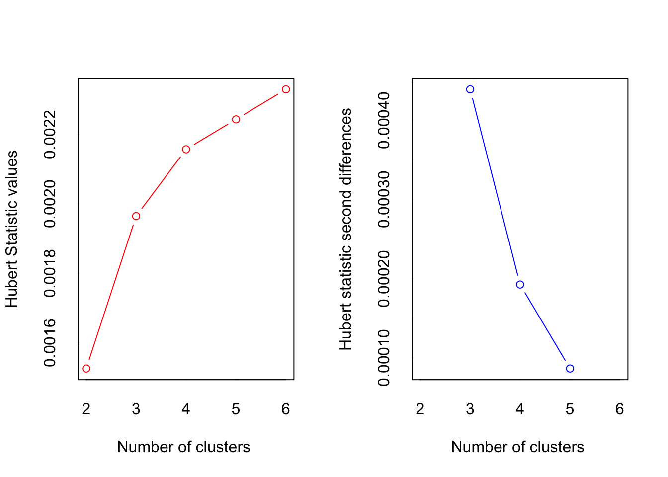
*** : The Hubert index is a graphical method of determining the number of clusters.
                In the plot of Hubert index, we seek a significant knee that corresponds to a
                significant increase of the value of the measure i.e the significant peak in Hubert
                index second differences plot.
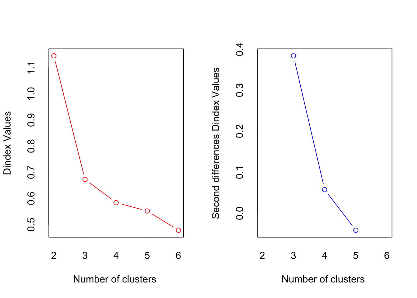
*** : The D index is a graphical method of determining the number of clusters.
                In the plot of D index, we seek a significant knee (the significant peak in Dindex
                second differences plot) that corresponds to a significant increase of the value of
                the measure.

*******************************************************************
* Among all indices:
* 2 proposed 2 as the best number of clusters
* 13 proposed 3 as the best number of clusters
* 8 proposed 4 as the best number of clusters

                   ***** Conclusion *****

* According to the majority rule, the best number of clusters is  3


*******************************************************************
# Get the best number of clusters based on the analysis
best_num_clusters <- result$Best.nc
# Display the best number of clusters
print(best_num_clusters) KL CH Hartigan CCC Scott Marriot TrCovW
Number_clusters 4.0000 4.0000 3.0000 3.0000 3.0000 3.0 3.000
Value_Index 54.0377 495.1816 171.9115 35.8668 276.8545 532302.7 6564.361
TraceW Friedman Rubin Cindex DB Silhouette Duda
Number_clusters 3.000 4.0000 4.0000 3.0000 3.0000 2.000 4.0000
Value_Index 117.076 151.3607 -32.3048 0.3163 0.7025 0.516 0.5932
PseudoT2 Beale Ratkowsky Ball PtBiserial Frey McClain Dunn
Number_clusters 4.0000 3.000 3.0000 3.0000 3.0000 1 2.0000 4.0000
Value_Index 32.9134 1.884 0.4922 87.7349 0.7203 NA 0.4228 0.1365
Hubert SDindex Dindex SDbw
Number_clusters 0 3.0000 0 4.0000
Value_Index 0 1.5717 0 0.1503Now that we have determined K, we are ready to cluster the data.
set.seed(20) #set the seed of the random number generator. Setting a seed allows you to reproduce random outcomes
kCluster <- kmeans(iris[, 3:4], 3, nstart = 50) #3 clusters for the 3 species, nstart = 50 for 50 different random starts and select the model with lowest variation
kCluster
K-means clustering with 3 clusters of sizes 50, 48, 52
Cluster means:
Petal.Length Petal.Width
1 1.462000 0.246000
2 5.595833 2.037500
3 4.269231 1.342308
Clustering vector:
[1] 1 1 1 1 1 1 1 1 1 1 1 1 1 1 1 1 1 1 1 1 1 1 1 1 1 1 1 1 1 1 1 1 1 1 1 1 1
[38] 1 1 1 1 1 1 1 1 1 1 1 1 1 3 3 3 3 3 3 3 3 3 3 3 3 3 3 3 3 3 3 3 3 3 3 3 3
[75] 3 3 3 2 3 3 3 3 3 2 3 3 3 3 3 3 3 3 3 3 3 3 3 3 3 3 2 2 2 2 2 2 3 2 2 2 2
[112] 2 2 2 2 2 2 2 2 3 2 2 2 2 2 2 3 2 2 2 2 2 2 2 2 2 2 2 3 2 2 2 2 2 2 2 2 2
[149] 2 2
Within cluster sum of squares by cluster:
[1] 2.02200 16.29167 13.05769
(between_SS / total_SS = 94.3 %)
Available components:
[1] "cluster" "centers" "totss" "withinss" "tot.withinss"
[6] "betweenss" "size" "iter" "ifault" Our clustering model did very well but, it’s important to note that in unsupervised learning methods like k-means clustering, the assigned cluster numbers don’t necessarily align with the original class labels. Therefore, interpretation of these clusters should be based on the patterns observed rather than direct mapping to the original classes, especially when dealing with real-world datasets where class labels are not available during clustering.
table(kCluster$cluster, iris$Species)
    setosa versicolor virginica
  1     50          0         0
  2      0          2        46
  3      0         48         4
# Plot iris clusters
kCluster$cluster <- as.factor(kCluster$cluster)
ggplot(iris, aes(Petal.Length, Petal.Width, color = kCluster$cluster)) + geom_point()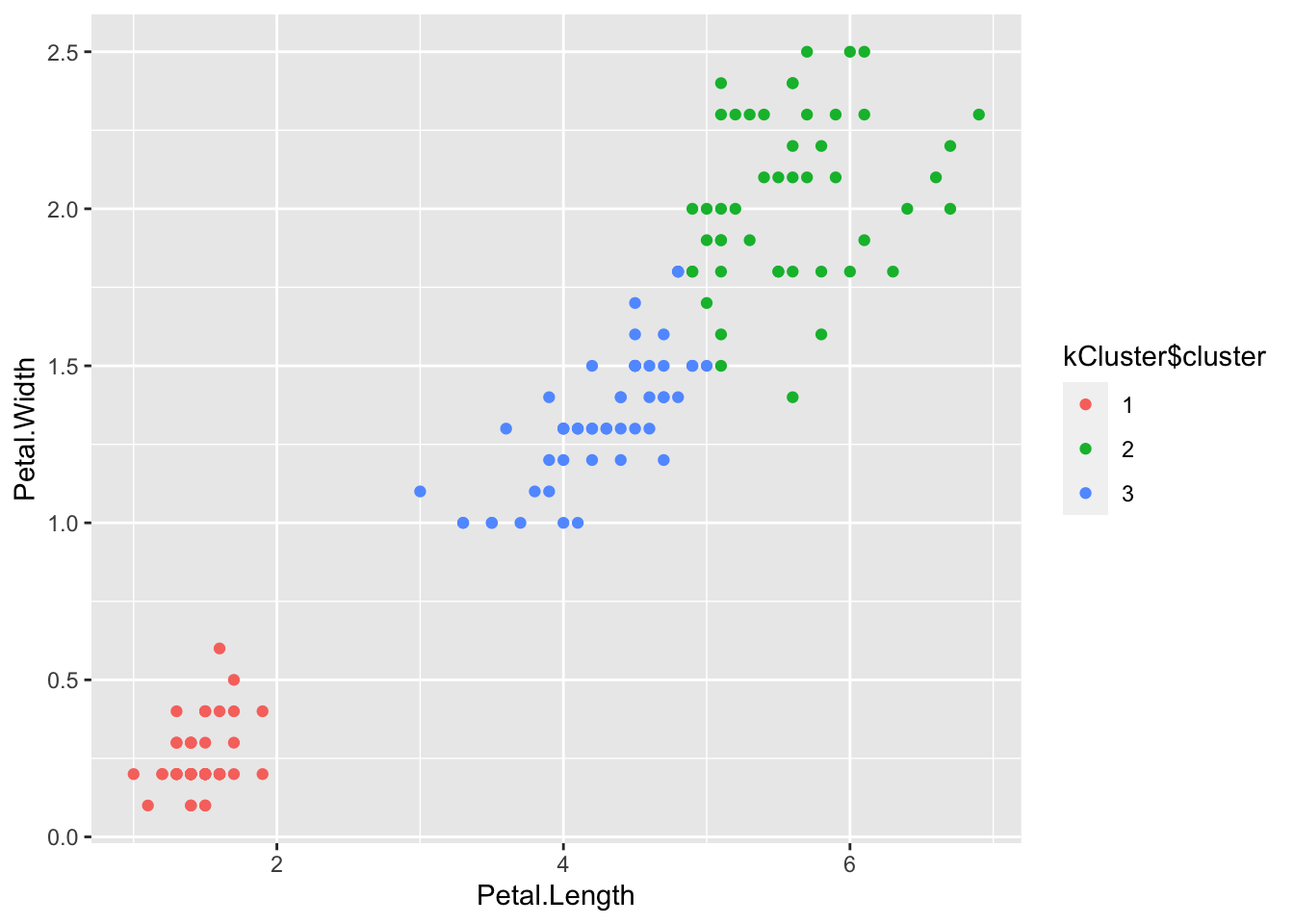
My belief [in contridiction to my mother’s belief ;) ]is that there is always more than one way to do something, and in this case I’m right. Another way to cluster data in R is to use a hierarchical approach.
# Cluster it using Hierarchical
Dist <- dist(iris, method="euclidean")
hiercluster <- hclust(Dist, method="average")
numcluster <- 3 #number of clusters
hCluster <- cutree(hiercluster, numcluster)

#contingency table
table(hCluster, iris$Species)
hCluster setosa versicolor virginica
       1     50          0         0
       2      0         50        14
       3      0          0        36
Now in graph form!
ggplot(iris, aes(Petal.Length, Petal.Width, color = hCluster)) + geom_point()
As always R while ugly and confusing at first glance makes data analysis a breeze! K-means clustering can be accomplished with a few lines of code and is a powerful unsupervised learning technique that enables data segmentation and pattern discovery without predefined categories. For those interested in further applications of its uses, check out tasks like customer segmentation, anomaly detection, and market analysis.